Kash’s Portfolio - Data Mining and EDA - Sound Stack Exchange Community

A Report by …

@Author: Kashish Mukheja

Introduction:

The Sound Stack Exchange platform serves as a hub for professionals, enthusiasts, and hobbyists interested in various aspects of sound technology, including audio production, sound design, acoustics, and music composition. In this project, we conduct an exploratory data analysis (EDA) of the Sound Stack Exchange community to gain insights into user behavior, content contributions, and community dynamics. Through the analysis of diverse datasets encompassing posts, comments, user profiles, and voting activities, we aim to uncover patterns, trends, and correlations that characterize the interactions within this specialized online community.

Abstract:

Our project delves into the rich dataset extracted from Sound Stack Exchange, a dedicated platform for individuals passionate about sound technology. We begin by merging multiple datasets, including information on posts, comments, users, votes, and badges, to form a comprehensive dataset for analysis. We then employ various data visualization techniques, statistical analyses, and exploratory methods to uncover valuable insights. These insights encompass the distribution of post topics, the engagement levels of users, the influence of badges on user behavior, and the temporal dynamics of community activity. Additionally, we explore the geographical distribution of users and their contributions, shedding light on the global reach of the Sound Stack Exchange community. Through our findings, we provide a deeper understanding of the dynamics and characteristics of this online platform, contributing to the broader discourse on digital communities and knowledge-sharing networks.

Import Libraries

We’ll start by importing the necessary libraries

import pandas as pd
import numpy as np
import xml.etree.ElementTree as ET
import csv
import seaborn as sns
from collections import Counter
from wordcloud import STOPWORDS
from wordcloud import WordCloud
import matplotlib.pyplot as plt
from IPython.display import display
import plotly.express as px
import re

Data Preparation

In this section, we detail the process of preparing the data which involves converting XML data into a structured CSV format, facilitating easier data analysis and manipulation. This phase includes the following steps:

XML Parsing: We’ll parse each XML file to extract the relevant data elements and their attributes.
Header Row Extraction: We’ll identify and extract the header rows from the XML files, ensuring that the CSV files have appropriate column names.
CSV Conversion: We’ll convert the parsed XML data into CSV format, where each row represents a record and each column corresponds to a data attribute.
Writing to CSV Files: Finally, we’ll write the converted data into CSV files, maintaining the integrity and structure of the original data.

# Define input and output file paths for Badges.xml
INPUT_FILE_BADGES_XML = "sound.stackexchange.com/Badges.xml"
OUTPUT_FILE_BADGES_CSV = "sound.stackexchange.com/Badges.csv"

# Define input and output file paths for Comments.xml
INPUT_FILE_COMMENTS_XML = "sound.stackexchange.com/Comments.xml"
OUTPUT_FILE_COMMENTS_CSV = "sound.stackexchange.com/Comments.csv"

# Define input and output file paths for PostLinks.xml
INPUT_FILE_POSTLINKS_XML = "sound.stackexchange.com/PostLinks.xml"
OUTPUT_FILE_POSTLINKS_CSV = "sound.stackexchange.com/PostLinks.csv"

# Define input and output file paths for PostHistory.xml
INPUT_FILE_POSTHISTORY_XML = "sound.stackexchange.com/PostHistory.xml"
OUTPUT_FILE_POSTHISTORY_CSV = "sound.stackexchange.com/PostHistory.csv"

# Define input and output file paths for Posts.xml
INPUT_FILE_POSTS_XML = "sound.stackexchange.com/Posts.xml"
OUTPUT_FILE_POSTS_CSV = "sound.stackexchange.com/Posts.csv"

# Define input and output file paths for Tags.xml
INPUT_FILE_TAGS_XML = "sound.stackexchange.com/Tags.xml"
OUTPUT_FILE_TAGS_CSV = "sound.stackexchange.com/Tags.csv"

# Define input and output file paths for Users.xml
INPUT_FILE_USERS_XML = "sound.stackexchange.com/Users.xml"
OUTPUT_FILE_USERS_CSV = "sound.stackexchange.com/Users.csv"

# Define input and output file paths for Votes.xml
INPUT_FILE_VOTES_XML = "sound.stackexchange.com/Votes.xml"
OUTPUT_FILE_VOTES_CSV = "sound.stackexchange.com/Votes.csv"

# Define input and output file paths
INPUT_FILES_XML = [
    INPUT_FILE_BADGES_XML,
    INPUT_FILE_COMMENTS_XML,
    INPUT_FILE_POSTLINKS_XML,
    INPUT_FILE_POSTHISTORY_XML,
    INPUT_FILE_POSTS_XML,
    INPUT_FILE_TAGS_XML,
    INPUT_FILE_USERS_XML,
    INPUT_FILE_VOTES_XML
]

OUTPUT_FILES_CSV = [
    OUTPUT_FILE_BADGES_CSV,
    OUTPUT_FILE_COMMENTS_CSV,
    OUTPUT_FILE_POSTLINKS_CSV,
    OUTPUT_FILE_POSTHISTORY_CSV,
    OUTPUT_FILE_POSTS_CSV,
    OUTPUT_FILE_TAGS_CSV,
    OUTPUT_FILE_USERS_CSV,
    OUTPUT_FILE_VOTES_CSV
]

def extract_header_rows(input_file):
    # Parse the XML file
    tree = ET.parse(input_file)
    root = tree.getroot()
    
    # Get the first row element
    first_row = root.find('row')
    
    # Extract attributes as header rows
    header_rows = [attr for attr in first_row.attrib]
    
    return header_rows

def parse_xml_to_csv(input_file, output_file, header_rows):
    # Parse the XML file
    tree = ET.parse(input_file)
    root = tree.getroot()
    
    # Open CSV file for writing
    with open(output_file, 'w', newline='', encoding='utf-8') as csvfile:
        writer = csv.writer(csvfile)
        
        # Write header row
        writer.writerow(header_rows)
        
        # Write data rows
        for row in root.findall('row'):
            data_row = [row.attrib.get(attr, '') for attr in header_rows]
            writer.writerow(data_row)

# Extract header rows from Badges.xml
header_rows = extract_header_rows(INPUT_FILE_COMMENTS_XML)
print(header_rows)

# Parse Badges.xml and convert to Badges.csv
parse_xml_to_csv(INPUT_FILE_COMMENTS_XML, OUTPUT_FILE_COMMENTS_CSV, header_rows)

['Id', 'PostId', 'Score', 'Text', 'CreationDate', 'UserId', 'ContentLicense']

# Loop through each XML file and convert to CSV
for input_file, output_file in zip(INPUT_FILES_XML, OUTPUT_FILES_CSV):
    # Extract header rows
    header_rows = extract_header_rows(input_file)
    print(f'header for {output_file} = {header_rows}')
    print()
    # Parse XML and convert to CSV
    parse_xml_to_csv(input_file, output_file, header_rows)

header for sound.stackexchange.com/Badges.csv = ['Id', 'UserId', 'Name', 'Date', 'Class', 'TagBased']

header for sound.stackexchange.com/Comments.csv = ['Id', 'PostId', 'Score', 'Text', 'CreationDate', 'UserId', 'ContentLicense']

header for sound.stackexchange.com/PostLinks.csv = ['Id', 'CreationDate', 'PostId', 'RelatedPostId', 'LinkTypeId']

header for sound.stackexchange.com/PostHistory.csv = ['Id', 'PostHistoryTypeId', 'PostId', 'RevisionGUID', 'CreationDate', 'UserId', 'Text', 'ContentLicense']

header for sound.stackexchange.com/Posts.csv = ['Id', 'PostTypeId', 'CreationDate', 'Score', 'ViewCount', 'Body', 'OwnerUserId', 'LastEditorUserId', 'LastEditDate', 'LastActivityDate', 'Title', 'Tags', 'AnswerCount', 'CommentCount', 'ContentLicense']

header for sound.stackexchange.com/Tags.csv = ['Id', 'TagName', 'Count']

header for sound.stackexchange.com/Users.csv = ['Id', 'Reputation', 'CreationDate', 'DisplayName', 'LastAccessDate', 'WebsiteUrl', 'Location', 'AboutMe', 'Views', 'UpVotes', 'DownVotes', 'AccountId']

header for sound.stackexchange.com/Votes.csv = ['Id', 'PostId', 'VoteTypeId', 'CreationDate']

Code Summary:

The provided code defines input and output file paths for a set of XML files and their corresponding CSV files. It then defines two functions: extract_header_rows and parse_xml_to_csv.

extract_header_rows:
- This function takes an input XML file path, parses the XML file, and extracts the attributes of the first row element as header rows.
- It returns a list of header rows extracted from the XML file.
parse_xml_to_csv:
- This function takes an input XML file path, an output CSV file path, and a list of header rows as arguments.
- It parses the XML file, extracts data from each row element, and writes the data into a CSV file.
- It writes the extracted header rows as the header row in the CSV file.

The code then iterates through each XML file and corresponding output CSV file. For each pair of files, it extracts the header rows using the extract_header_rows function and then parses the XML file and converts it to a CSV file using the parse_xml_to_csv function.

Benefits of the Code:

Modular and Reusable: The code is modularized into functions, making it easy to reuse for different XML files.
Automated Conversion: The code automates the conversion process, eliminating the need for manual conversion of XML files to CSV.
Maintains Data Integrity: The code ensures that the structure and integrity of the data are maintained during the conversion process.

Overall, this code efficiently converts XML files to CSV format, providing a convenient way to work with structured data in a tabular format.

# Load Badges.csv into a pandas DataFrame
df_badges = pd.read_csv(OUTPUT_FILE_BADGES_CSV)

# Load Comments.csv into a pandas DataFrame
df_comments = pd.read_csv(OUTPUT_FILE_COMMENTS_CSV)

# Load PostLinks.csv into a pandas DataFrame
df_postlinks = pd.read_csv(OUTPUT_FILE_POSTLINKS_CSV)

# Load PostHistory.csv into a pandas DataFrame
df_posthistory = pd.read_csv(OUTPUT_FILE_POSTHISTORY_CSV)

# Load Posts.csv into a pandas DataFrame
df_posts = pd.read_csv(OUTPUT_FILE_POSTS_CSV)

# Load Tags.csv into a pandas DataFrame
df_tags = pd.read_csv(OUTPUT_FILE_TAGS_CSV)

# Load Users.csv into a pandas DataFrame
df_users = pd.read_csv(OUTPUT_FILE_USERS_CSV)

# Load Votes.csv into a pandas DataFrame
df_votes = pd.read_csv(OUTPUT_FILE_VOTES_CSV)

Data Merging:

The code starts by merging several DataFrames using the pd.merge() function. Each merge operation combines DataFrames based on specified conditions, such as matching columns or keys. The suffixes parameter is used to differentiate columns from different DataFrames in the merged result.

# Merge the dataframes
merged_df = pd.merge(df_posts, df_comments, how='left', left_on='Id', right_on='PostId', suffixes=('_posts', '_comments'))
merged_df = pd.merge(merged_df, df_posthistory, how='left', left_on='Id_posts', right_on='PostId', suffixes=('', '_post_history'))
merged_df = pd.merge(merged_df, df_postlinks, how='left', left_on='Id_posts', right_on='PostId', suffixes=('', '_post_links'))
merged_df = pd.merge(merged_df, df_users, how='left', left_on='OwnerUserId', right_on='Id', suffixes=('', '_users'))
merged_df = pd.merge(merged_df, df_votes, how='left', left_on='Id_posts', right_on='PostId', suffixes=('', '_votes'))
merged_df = pd.merge(merged_df, df_badges, how='left', left_on='Id_posts', right_on='Id', suffixes=('', '_badges'))

merged_df.head()

	Id_posts	PostTypeId	CreationDate_posts	Score_posts	ViewCount	Body	OwnerUserId	LastEditorUserId	LastEditDate	LastActivityDate	...	Id_votes	PostId_votes	VoteTypeId	CreationDate_votes	Id_badges	UserId_badges	Name	Date	Class	TagBased
0	18	1	2010-02-22T16:46:22.670	1	8731.0	<p>I just did the tutorial "<a href="http://ww...	4.0	6957.0	2015-10-11T13:55:00.060	2015-10-11T13:55:00.060	...	22.0	18.0	2.0	2010-02-22T00:00:00.000	18.0	10.0	Teacher	2010-03-02T07:22:12.013	3.0	False
1	18	1	2010-02-22T16:46:22.670	1	8731.0	<p>I just did the tutorial "<a href="http://ww...	4.0	6957.0	2015-10-11T13:55:00.060	2015-10-11T13:55:00.060	...	22.0	18.0	2.0	2010-02-22T00:00:00.000	18.0	10.0	Teacher	2010-03-02T07:22:12.013	3.0	False
2	18	1	2010-02-22T16:46:22.670	1	8731.0	<p>I just did the tutorial "<a href="http://ww...	4.0	6957.0	2015-10-11T13:55:00.060	2015-10-11T13:55:00.060	...	22.0	18.0	2.0	2010-02-22T00:00:00.000	18.0	10.0	Teacher	2010-03-02T07:22:12.013	3.0	False
3	18	1	2010-02-22T16:46:22.670	1	8731.0	<p>I just did the tutorial "<a href="http://ww...	4.0	6957.0	2015-10-11T13:55:00.060	2015-10-11T13:55:00.060	...	22.0	18.0	2.0	2010-02-22T00:00:00.000	18.0	10.0	Teacher	2010-03-02T07:22:12.013	3.0	False
4	18	1	2010-02-22T16:46:22.670	1	8731.0	<p>I just did the tutorial "<a href="http://ww...	4.0	6957.0	2015-10-11T13:55:00.060	2015-10-11T13:55:00.060	...	22.0	18.0	2.0	2010-02-22T00:00:00.000	18.0	10.0	Teacher	2010-03-02T07:22:12.013	3.0	False

5 rows × 57 columns

Duplicate Column Check:

After merging, the code checks for the presence of duplicate columns in the merged DataFrame using the duplicated() method. If duplicate columns are found, they are removed from the DataFrame using the loc accessor with a boolean mask to select only non-duplicate columns. Finally, the shape of the DataFrame is printed to confirm the removal of duplicate columns.

# check for the presence of duplicates
duplicate_columns = merged_df.columns[merged_df.columns.duplicated()]
if len(duplicate_columns) > 0:
    print(f'Duplicate columns found: {duplicate_columns}')
    merged_df = merged_df.loc[:,~merged_df.columns.duplicated()]
    merged_df.shape
else:
    print(f'No duplicates columns found!')

No duplicates columns found!

This code snippet effectively combines disparate datasets into a single coherent DataFrame and ensures data integrity by removing any duplicate columns that may have resulted from the merging process.

Top 10 Tags Analysis

Summary:

In this visualization, we aim to analyze the top 10 tags present in the dataset. The process involves extracting tags from the ‘Tags’ column of the merged DataFrame, counting the occurrences of each tag, and plotting the top 10 tags in a bar chart.

By examining the frequency of tags, we gain insights into the most commonly associated topics or themes within the dataset. This analysis helps in understanding the prevalent subjects of discussion or interest among users contributing to the dataset.

# viz 1
# Search for the top 10 tags in the data
tags = merged_df['Tags'].dropna().apply(lambda x: re.findall(r'<(.*?)>', str(x)))
all_tags = [tag for sublist in tags for tag in sublist]

# Create the df
tag_df = pd.DataFrame({'Tag': all_tags})

# Plot top tags
top_tags = tag_df['Tag'].value_counts().nlargest(10)
plt.figure(figsize=(12, 6))
sns.barplot(x=top_tags.values, y=top_tags.index, palette='viridis')
plt.title('Top 10 Tags')
plt.xlabel('Count')
plt.ylabel('Tag')
plt.show()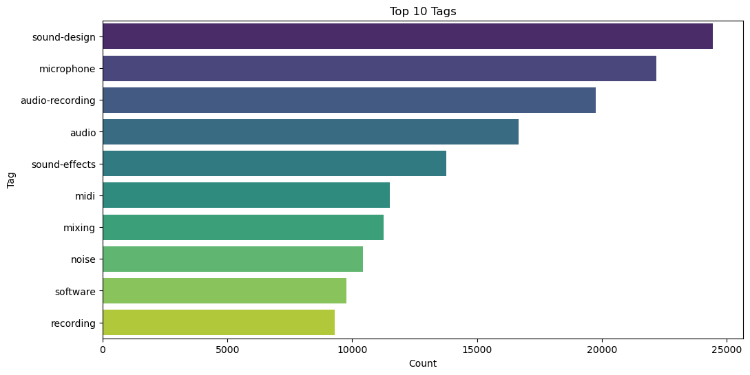

Top Users Contribution Analysis

Summary:

This visualization focuses on identifying and analyzing the top users based on their contributions to the dataset. Initially, we extract the counts of posts associated with each user’s display name and visualize the distribution using a pie chart.

The pie chart provides a visual representation of the relative contributions of the top 10 users, allowing us to quickly identify the most active participants in the dataset.

Subsequently, we filter the data to include only the posts made by the top users and create a pivot table. This pivot table summarizes the average score and view count for each of the top users.

By examining the average scores and view counts, we gain insights into the quality and popularity of the posts made by the top contributors. This analysis helps in recognizing the most influential and impactful users within the dataset.

# Get the top users and their post counts
top_users_counts = merged_df['DisplayName'].value_counts().nlargest(10)

# Visualize top users based on their contribution
plt.figure(figsize=(8, 8))
plt.pie(top_users_counts, labels=top_users_counts.index, autopct='%1.1f%%', startangle=140)
plt.title('Top 10 Users Contribution')
plt.show()

# Filter data for top users
filtered_data_top_users = merged_df[merged_df['DisplayName'].isin(top_users_counts.index)]

# Create a pivot table showing the average Score_posts and ViewCount for each top user
pivot_table_top_users = pd.pivot_table(filtered_data_top_users, values=['Score_posts','ViewCount'], index='DisplayName', aggfunc='mean')

# Handle non-finite values in the 'ViewCount' column and convert it to integers
pivot_table_top_users['ViewCount'] = pivot_table_top_users['ViewCount'].fillna(0).replace([np.inf, -np.inf], 0)
pivot_table_top_users['ViewCount'] = pivot_table_top_users['ViewCount'].astype(int)

# Sort the pivot table by 'Score_posts' column in descending order
pivot_table_top_users = pivot_table_top_users.sort_values(by='Score_posts', ascending=False)

# Rename columns for clarity
pivot_table_top_users = pivot_table_top_users.rename(columns={'Score_posts': 'Avg_Score_posts',
                                                             'ViewCount': 'Avg_ViewCount'})

# Display the pivot table
display(pivot_table_top_users)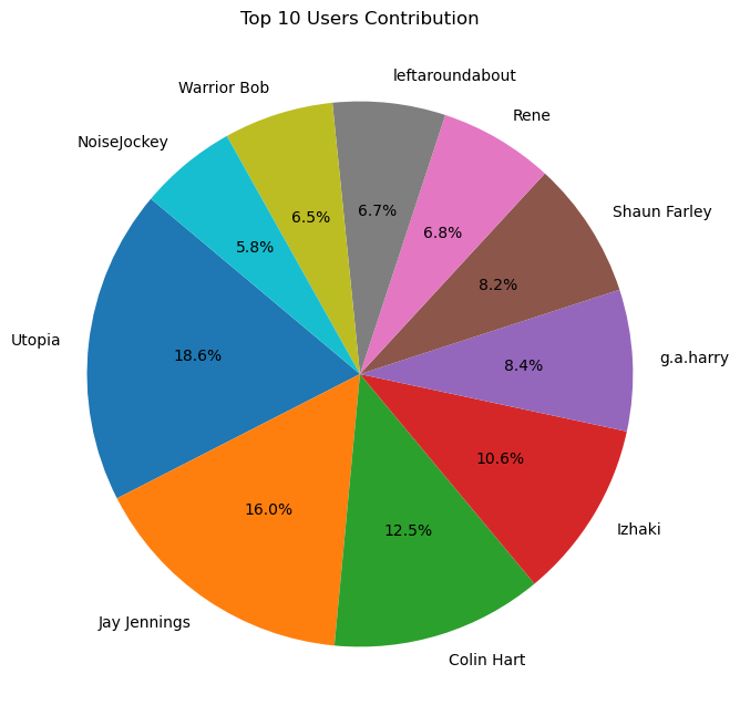

	Avg_Score_posts	Avg_ViewCount
DisplayName
Izhaki	47.292579	0
Colin Hart	13.350414	4178
leftaroundabout	12.540337	0
Warrior Bob	9.740613	1786
Jay Jennings	8.923619	2947
Utopia	8.247516	8159
g.a.harry	7.605453	1928
Shaun Farley	7.260140	965
Rene	6.379020	1733
NoiseJockey	6.125487	2989

Data Analysis: Locations Insights

Summary:

This section focuses on analyzing the data based on the locations provided by users. Initially, we filter the dataset to include only records with non-null location information.

Afterwards, we convert the creation dates of various entities to datetime objects to facilitate further analysis. This step ensures consistency and avoids potential warnings.

Next, we calculate several metrics to gain insights into the posting behavior and engagement levels of users from different locations. The metrics include: - Posts per day: Average number of posts made by users from each location per day. - Average Post Score: The average score received by posts from each location. - Average Views: The average number of views received by posts from each location.

Subsequently, we create a summary table aggregating the calculated metrics for each unique location. This summary table provides a comprehensive overview of the posting activity and engagement levels across different locations.

Finally, we visualize the top 20 locations with the highest number of posts using Plotly Express. This visualization helps in identifying the most active regions in terms of user contributions, facilitating further analysis and insights into regional posting trends.

# data with location

Location_df = merged_df[~merged_df['Location'].isna()]
len(Location_df)

pd.options.mode.chained_assignment = None

# Convert creation dates to datetime objects to avoid SettingWithCopyWarning
Location_df['CreationDate_posts'] = pd.to_datetime(Location_df['CreationDate_posts'])
Location_df['CreationDate_comments'] = pd.to_datetime(Location_df['CreationDate_comments'])
Location_df['CreationDate_post_links'] = pd.to_datetime(Location_df['CreationDate_post_links'])
Location_df['CreationDate_users'] = pd.to_datetime(Location_df['CreationDate_users'])
Location_df['CreationDate_votes'] = pd.to_datetime(Location_df['CreationDate_votes'])

# Calculate the metrics
Location_df['Posts per Day'] = Location_df['Id_posts'] / (pd.to_datetime('today') - Location_df['CreationDate_posts']).dt.days
Location_df['Average PostScore'] = Location_df['Score_posts'] / Location_df['Id_posts']
Location_df['Average Views'] = Location_df['Views'] / Location_df['Id_posts']

# Create a summary table
location_summary = Location_df.groupby('Location').agg({
    'Id_posts': 'count',
    'OwnerUserId': 'nunique',
    'Posts per Day': 'mean',
    'Average PostScore': 'mean',
    'Views': 'sum'
}).reset_index()

# Rename columns for clarity
location_summary.columns = ['Location', 'Posts', 'Unique Contributors', 
                            'Avg Posts/Day', 'Avg Post Score', 'Total Views']

# Display the top 20 locations by number of posts
location_summary_top20 = location_summary.sort_values(by='Posts', ascending=False).head(20)
location_summary_top20

	Location	Posts	Unique Contributors	Avg Posts/Day	Avg Post Score	Total Views
186	California	16107	19	2.540462	0.001894	24209550.0
553	London	11253	38	5.916709	0.001239	617825.0
187	California, USA	9230	1	2.162928	0.003015	15875600.0
755	Orlando, Fl	7240	1	0.417693	0.020865	5473440.0
1053	Toronto	5699	6	3.089592	0.000879	3235560.0
109	Berkeley, CA	5395	4	2.333486	0.001545	5830905.0
249	Dallas	3954	2	2.577033	0.001031	1955118.0
108	Bergen, Norway	3855	1	7.220469	0.000467	589815.0
567	Los Angeles, CA	3839	15	2.052593	0.001289	2954372.0
1084	United Kingdom	3786	48	12.205236	0.000331	37748.0
559	London, United Kingdom	3751	37	41.929947	0.000093	410664.0
893	San Francisco Bay Area	3339	1	1.169286	0.010128	2958354.0
928	Seattle, WA	3289	15	6.075481	0.000223	194267.0
447	Illinois	3107	3	5.285660	0.000795	31004.0
614	Melbourne, Australia	3029	12	25.227580	0.002393	495537.0
33	Amsterdam, Netherlands	2957	8	2.015193	0.016708	2550107.0
837	Rensselaer, NY	2915	1	8.431776	0.000121	638385.0
346	France	2825	22	2.716287	0.001992	1196140.0
64	Auckland, New Zealand	2721	5	1.650918	0.001601	803128.0
737	Odense, Denmark	2639	1	14.429640	0.000116	398489.0

# Create a bar chart for posts by location
fig = px.bar(
    location_summary_top20,
    x='Location',
    y='Posts',
    title='Top 20 Locations by Posts',
    height=600,
    category_orders={'Location': location_summary_top20['Location']},
    text='Location',
    color='Location'  # Change the color of bars based on location
)

# Rotate x-axis labels for better readability
fig.update_layout(xaxis_tickangle=-45)

# Show the bar chart
fig.show()

Data Visualization: Posts by Location Insights

Summary:

This section presents a bar chart visualization illustrating the distribution of posts across the top 20 locations with the highest posting activity.

Using Plotly Express, we create a bar chart where each bar represents a specific location, and its height corresponds to the number of posts contributed from that location. The color of the bars is also determined by the location, aiding in visually distinguishing between different regions.

To enhance readability, we rotate the x-axis labels by -45 degrees, ensuring that location names are displayed more clearly and prevent overlap.

The resulting visualization provides a clear and intuitive representation of the posting activity across different locations, allowing for easy comparison and identification of the most active regions in terms of user contributions.

Analyzing Post Frequency Over Time

Summary:

This section explores the frequency of postings over time by analyzing the monthly post counts.

We begin by converting the ‘CreationDate_posts’ column to datetime format and setting it as the index of the dataframe. This allows us to easily perform time-based operations.

Next, we use the resample function to aggregate the post counts on a monthly basis. By specifying the parameter 'M', we group the data into monthly intervals.

A line plot is then generated, where each data point represents the count of posts made in a particular month. The x-axis represents time, while the y-axis indicates the corresponding number of posts.

# Checking how many postings were made over the period of time
merged_df['CreationDate_posts'] = pd.to_datetime(merged_df['CreationDate_posts'])
merged_df.set_index('CreationDate_posts', inplace=True)

plt.figure(figsize=(15, 6))
merged_df.resample('M').size().plot(legend=False)
plt.title('Monthly Post Count Over Time')
plt.xlabel('Date')
plt.ylabel('Number of Posts')
plt.show()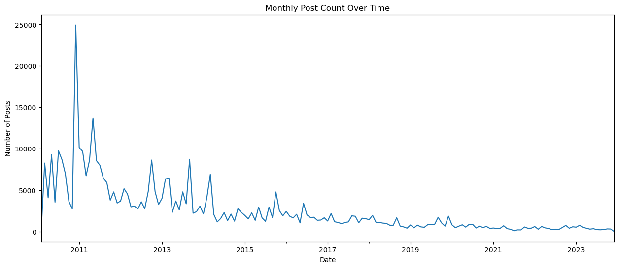

This visualization provides insights into the posting trends over the period under analysis, highlighting any significant changes or patterns in posting activity over time.

Conclusion:

In conclusion, our exploratory data analysis of the Sound Stack Exchange community has revealed intriguing patterns and trends inherent within the platform. We have observed the dominance of certain topics, the active participation of a subset of users, and the impact of badges on incentivizing contributions. Additionally, our analysis of temporal trends and geographical distributions has provided valuable insights into the evolution and diversity of the community. By uncovering these insights, we not only enhance our understanding of the Sound Stack Exchange platform but also contribute to the broader body of knowledge on online communities and collaborative platforms. Our findings underscore the importance of data-driven approaches in elucidating the dynamics of digital communities and highlight avenues for further research and exploration in this domain.

Introduction:

Abstract:

Import Libraries

Data Preparation

Code Summary:

Benefits of the Code:

Data Merging:

Duplicate Column Check:

Top 10 Tags Analysis

Top Users Contribution Analysis

Data Analysis: Locations Insights

Data Visualization: Posts by Location Insights

Analyzing Post Frequency Over Time

Conclusion:

Thank You for Reading the Report